UNG: Why Pure Gasoline ETFs May Disappoint (Technical Evaluation) (NYSEARCA:UNG)

Pure gasoline costs are down about 80% from their highs 9 months in the past and down 60% from their ranges solely 5 months in the past. This has probably contributed to sluggishness in pure gasoline shares, as evidenced by the efficiency of the First Belief Pure Gasoline ETF (FCG) over that very same time frame. Unsurprisingly, the collapse in pure gasoline costs is mirrored within the abysmal efficiency of commodity-tracking ETFs just like the United States Pure Gasoline Fund, LP ETF (NYSEARCA:UNG) and the US 12 Month Pure Gasoline Fund, LP ETF (UNL).

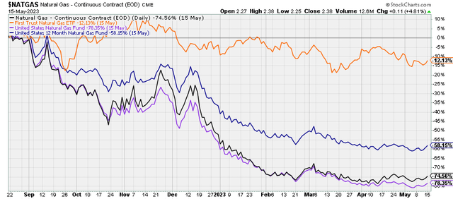
On this article, I’m going to argue in the direction of the next conclusions:

Pure gasoline costs are more likely to see a considerable rise over the subsequent 16-24 months. Neither UNG nor UNL are, at current, good devices to make the most of such an increase as a result of pronounced contango within the pure gasoline market in the meanwhile.

That is primarily based on an analyses of commodity cycle dynamics inside present macro situations and the historical past of pure gasoline costs during the last 60 years.

In a subsequent article, I intend to argue that, though pure gasoline costs are more likely to stabilize if not rise:

Pure gasoline equities – significantly within the exploration and manufacturing house, comparable to these represented in FCG – should not more likely to considerably profit from even a doubling of costs. Over the long term, pure gasoline shares are more likely to outperform the broader fairness market and exchange-traded funds, or ETFs, like UNG and UNL, however they’re more likely to undergo from a interval of low absolute returns.

For now, nevertheless, let’s start with the outlook for pure gasoline costs.

Commodity rules

In December, I wrote “DBE ETF: Vitality Costs Probably To Begin Main Market Down.” I argued there that markets, together with commodity markets, have probably entered a “secular” interval of decrease returns and that we’re in all probability in a cyclical downturn inside that “secular” bear market. That cyclical downturn could be anticipated to final no less than till 2024 whereas a extra common interval of depressed returns might final effectively into the 2030s. Within the meantime, I argued, vitality costs have been more likely to really feel the brunt of that cyclical downturn, extra so than treasured metals, industrial metals, and agricultural commodities. To this point, there has not been a lot motive to vary that common outlook on vitality, however it seems that pure gasoline could also be considerably oversold now, and the underlying rationale behind the vitality outlook factors to an idiosyncratic trajectory for pure gasoline. In different phrases, we’re more likely to see stabilization in pure gasoline costs earlier than we see it in the remainder of the vitality advanced.

I’ve described the strategy that will probably be employed right here in higher element in earlier articles, together with a common piece on commodities in March of final yr. For now, nevertheless, I’ll briefly recap a few of these parts and the way they relate to pure gasoline costs.

We will divide commodity worth conduct into structural, tremendous cyclical, and cyclical tendencies. Structurally, commodity costs collectively are typically flat over centuries, and individually they have an inclination to comply with a easy method: worth = 1/provide, which means that worth isn’t pushed primarily by supply-demand dynamics.

Reasonably, actual commodity costs have been persistently correlated with the earnings yield on equities for the final 150 years. Because the chart illustrates beneath, this has been much less true for pure gasoline costs (presumably as a result of it isn’t as fungible as most different main commodities).

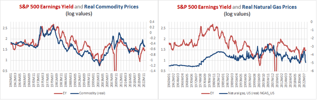
On high of this, decade-long commodity tremendous cycles happen in periods marked by elevated international instability (as mirrored in international deaths in battle) and intervals which can be marked by the transition from one dominant technological paradigm to a different. This was mentioned in higher element within the collection Conjunction & Disruption: Expertise, Conflict, And Asset Costs. On the flip facet, commodity costs are typically depressed in periods of rising PEs, rising international stability, and the diffusion part of a disruptive innovation (for instance, autos and radios, TVs, PCs, smartphones).

And, because the institution of the Federal Reserve, tremendous cyclical waves in commodity costs (and the phenomena related to them) have occurred each 30 years (for instance, the 1910s, Forties, Seventies, and 2000s). Aside from a couple of particulars, that is the fashionable type of Kondratiev Waves, as mentioned in that collection.

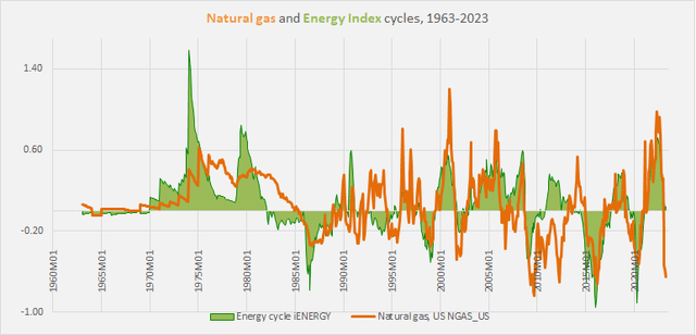
Lastly, commodity costs even have a cyclical mode of conduct. Usually, they rise and fall with company earnings and rates of interest. They have an inclination to peak each three to 5 years. In addition they have what we’d name a commodity curve. That’s, treasured metals rise earlier than industrial metals, which rise earlier than agricultural commodities (most notably grains), which rise earlier than vitality costs. Industrial metals are most carefully aligned with the earnings cycle, which seems to kind the core of the bigger market cycle.

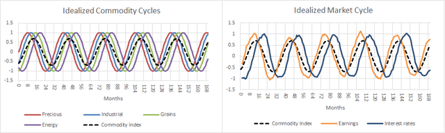
By monitoring tremendous cyclical and cyclical situations, that are pushed by fundamentals outdoors of the present scope of present financial idea, I believe that we are able to anticipate strikes in numerous asset lessons, together with commodities.

For instance, on the cyclical degree, the ratio of treasured metals costs to these of a given commodity tends to foretell the following conduct of that commodity. That’s illustrated within the chart beneath.

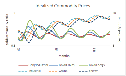
Due to the character of the commodity curve, a excessive gold worth (gold is the dear steel par excellence) relative to a different commodity probably signifies that that commodity will rise over the subsequent 16 months or so. Equally, a low gold worth ratio means that commodity will decline over the subsequent 16 months or so.

Gold as a number one indicator

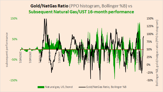
That is illustrated within the following two charts. The primary chart compares the gold/pure gasoline ratio (in crimson) with the following efficiency of pure gasoline costs (in blue). The second chart compares the Bollinger %B technical indicator for the gold/pure gasoline ratio (in black) alongside the following efficiency of the ratio of pure gasoline costs to 10-year Treasury bond returns (in inexperienced). The place the %B indicator equals 100%, the gold/pure gasoline ratio has moved two commonplace deviations up. The place it’s 0%, the ratio has moved two commonplace deviations down. In latest weeks, the %B indicator has been in extra of 100%.

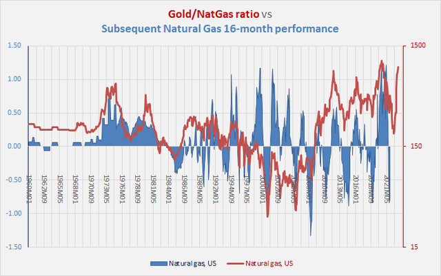
This works higher with some lessons of commodities (for instance, grains) higher than different lessons (for instance, drinks) and inside lessons, this works higher with some commodities (for instance, tea) than others (for instance, cocoa). Realizing that market cycles are likely to final three to 5 years additionally helps us create further methods to measure the standing of a given cycle, and understanding that yields are correlated with different parts of the market cycle permits us to amplify the cycle by performances relative to Treasury bonds.

As the present downcycle ages, some commodities are more likely to get to the underside prior to others. A kind of seems to be pure gasoline. However, pure gasoline behaves in quite uncommon methods.

Pure gasoline cycles

First, as illustrated in Chart B above, pure gasoline has not obeyed the dictates of the earnings yield-commodity correlation in addition to different commodities have. Second, its cyclicality is considerably erratic. Within the following charts, I distinction the pure gasoline cycles with the economic metals cycle, the earnings cycle, and the vitality cycle.

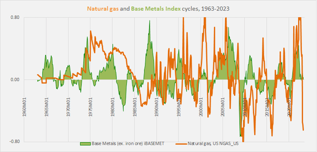
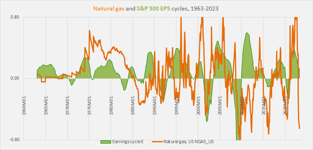
The pure gasoline cycle has more and more marched in line with the vitality cycle, though it may nonetheless expertise excessive short-term volatility. The vitality index above is calculated utilizing World Financial institution fixed weights, with pure gasoline’s contribution solely coming in at 10%, so this elevated correlation is unlikely to be as a result of direct influence of pure gasoline costs.

As with different commodities, the gold ratio has been a usually dependable predictor of subsequent pure gasoline efficiency, significantly when the gold/pure gasoline ratio makes excessive strikes. That is proven within the following chart, the place we see the gold/pure gasoline ratio on the high and the histogram of the proportion worth oscillator within the center overlaid with a Bollinger band. The underside panel of the chart exhibits pure gasoline costs to point out the connection between excessive strikes within the gold/pure gasoline ratio and pure gasoline costs themselves.

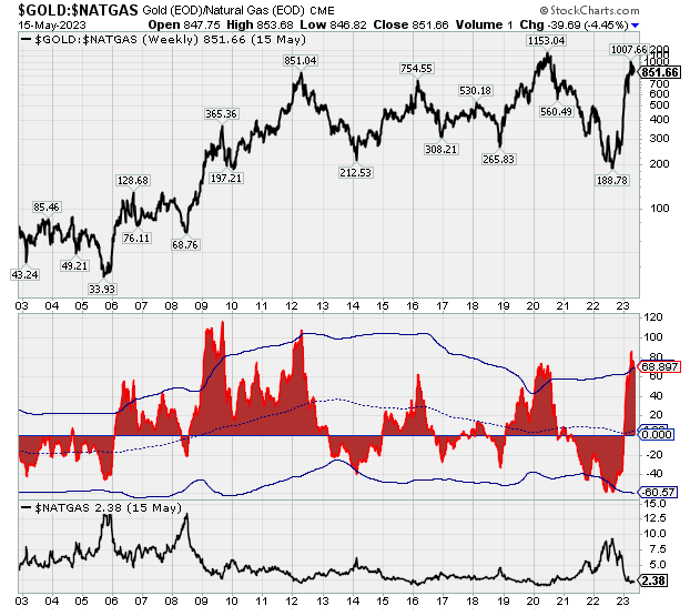
At present, the extraordinarily excessive momentum within the gold/pure gasoline ratio (due to each a powerful gold efficiency and distinctive weak spot in pure gasoline) means that we’re nearing a backside in pure gasoline costs. During the last 60 years, excessive strikes within the gold/pure gasoline ratio have resulted in roughly 75% upside in pure gasoline over the next 16 months, give or take 75%. That’s, in 16 months’ time, a variety for pure gasoline costs someplace between $2.00 and $5.50 can be regular.

For somebody who’s extraordinarily obese a downcycle situation for markets, that is a sexy proposition, because it probably permits one to hedge towards these deflationary bets. However, as I’ll attempt to present, it’s tough to place this thesis into observe.

One motive is that the volatility of pure gasoline costs makes it much less amenable to straightforward cyclical measures. For instance, one of the best outcomes for beating each the pure gasoline, utilizing month-to-month spot information from the World Financial institution, and 10-year Treasury bond markets during the last sixty years was buying and selling with adjustments to the fickle 16-month fee of change. Even this was solely barely higher than shopping for and holding Treasuries.

The next chart exhibits pure gasoline costs within the high column adopted by three measures of estimating 16-month (or 69-week) momentum.

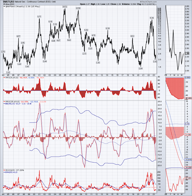
Theoretically, leaping between pure gasoline and 10-year Treasury bonds with each shift within the 16-month fee of change would enable one to beat a (theoretical) buy-and-hold technique, and during the last 5 months, there does appear to be a positive shift in momentum.

The issue is, even assuming that this technique is dependable and that pure gasoline costs are certainly about to enter a brand new bull market, how can we specific this within the type of a commerce or funding? I don’t assume it’s particularly sensible.

The pure gasoline futures curve

Historical past means that two situations usually want to carry to extend one’s probabilities of getting cash in pure gasoline ETFs:

Spot costs must rise. The futures curve must be inverted or comparatively flat.

However, it is a tough needle to string, as a result of the futures curve (usually, the unfold between long-dated futures and spot costs) usually strikes in the wrong way as spot costs. In different phrases, futures curves are most definitely to be inverted when spot costs are peaking, and when spot costs are bottoming, the futures curve is most definitely to be steep.

I’m going to briefly evaluation the connection between spot costs and futures after which how that performs out on the degree of the UNG and UNL ETFs. The futures curve evaluation will depend on month-to-month information supplied by the US Vitality Info Administration on spot and futures costs for the following 4 months’ contracts because the mid-Nineties. That historical past is illustrated beneath.

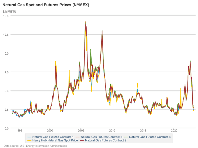
Usually, futures shadow spot costs fairly carefully.

The next chart exhibits futures curves calculated in 3 ways, the log of the ratio between the fourth supply month’s futures worth (i.e., “Contract 4”) and the spot worth, the log of the ratio the fourth and first supply month’s futures costs (i.e., “Contract 4” and “Contract 1”), and the slope of the log of all costs from spot by means of to Contract 4 costs.

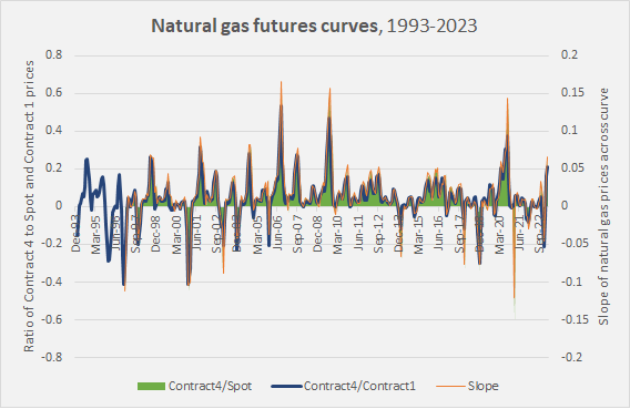
The log ratios are roughly equal to proportion values. That’s, if the Contract 4/Spot ratio is 0.60, that’s roughly equal to saying that Contract 4 costs are 60% greater than spot costs. For instance, in accordance with the chart above, which works as much as March of this yr, Contract 4 was about 20% greater than spot costs.

Usually, from this attitude, it doesn’t seem that it issues exactly the way you calculate the curve. You’ll broadly finish with comparable outcomes. We will usually use the ratio of Contract 4 to identify costs as our proxy for situations alongside the curve, with the caveat that this doesn’t embrace any longer-dated contracts. This caveat might matter when coping with UNL, because it holds contracts unfold out over a 12-month interval.

The next chart locations the futures curve alongside the spot and Contract 1 costs.

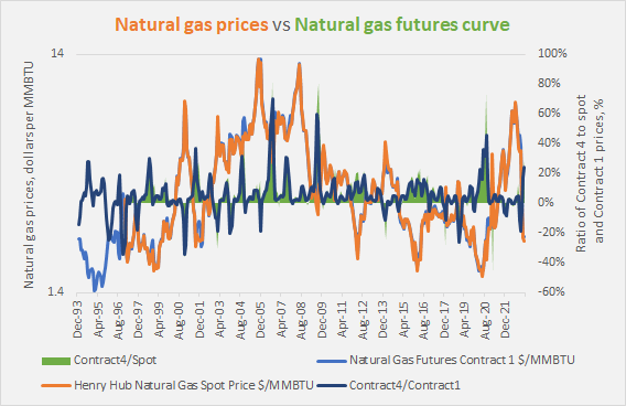
The next chart exhibits rolling correlations between pure gasoline costs and the curve.

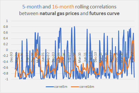
Usually, these correlations are unfavourable, that means that adjustments in spot costs have a tendency transfer the curve. It’s tough to seek out conditions during which costs are low and the futures curve is in backwardation or flat.

Pure gasoline ETFs and futures curves

UNG primarily invests within the near-month pure gasoline futures contracts, which suggests it usually has to roll contracts on a month-to-month foundation. In a market which is sort of all the time in contango, because of this UNG will usually have a better roll yield than UNL. UNL invests in pure gasoline futures contracts for the present month and the subsequent 11 months, and every month, it replaces the expired contract with a brand new one from a yr forward, maintaining a continuing 12-month unfold of contracts. This lowers draw back danger over the long run on common. Below sure situations, significantly when pure gasoline costs are in free fall and the market is heading into steep contango, it permits you to “beat” spot costs.

Thus, within the following chart which exhibits pure gasoline spot costs (in black) alongside the ratio of UNG (in inexperienced) and UNL (in orange) to identify costs, you possibly can see that the orange line usually rises because the black line falls, however each UNG and UNL usually severely underperform spot costs.

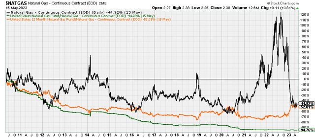
UNG and UNL have been round since 2007 and 2009, respectively, roughly on the tail finish of the commodity tremendous cycle, and I used to be curious if these ETFs may repay in an excellent cycle regardless of their continual underperformance relative to identify costs, so I approximated the efficiency of three theoretical funds that began in 1994, illustrated within the chart beneath.

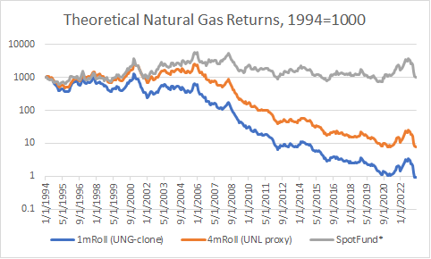
The “SpotFund” assumes which you can spend money on pure gasoline spot costs (for the interval up till January 1997, I substituted Contract 1 costs for the lacking spot costs). “1mRoll” rolls the near-term contract a lot in the way in which UNG does, and “4m Roll” sells the near-term contract every month to purchase Contract 4, a lot in the identical method that UNL does, though UNL would probably outperform this proxy, as a result of its contracts are unfold out over twelve months quite than 4.

The next chart compares the try and approximate UNG returns with UNG’s precise efficiency.

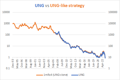
Early on, up till the primary spike in pure gasoline costs in 1999-2000, these theoretical futures funds sustain with spot costs comparatively effectively, however as contango grew to become extra pronounced, returns in these funds fell additional and additional behind.

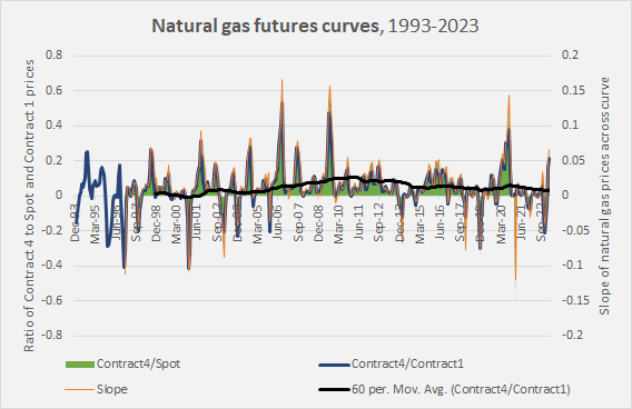
The next chart exhibits that as contango steepened over the course of the tremendous cycle of the 2000s, relative fund efficiency plunged.

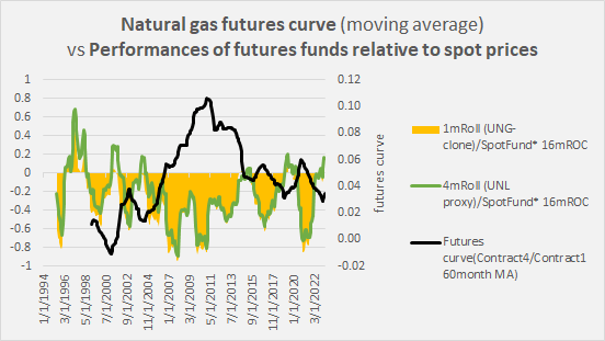
The last word level, nevertheless, is to not beat spot costs however to easily earn a living. If you will get 33% of a 6x transfer and cut back danger, that’s what issues.

So, to not belabor the purpose, there’s a sample that appears to maximise probabilities of getting a piece of pure gasoline upcycles. I’ll attempt to illustrate this utilizing the earlier cycle that kicked off in 2020.

The 2020-2022 upcycle

The next chart for the years 2018-2022 exhibits pure gasoline spot costs in purple, UNG in inexperienced, and UNL in orange within the high panel. It exhibits the UNG/UNL ratio in brown within the second panel, and it exhibits one measure of spot worth momentum in purple on the third panel.

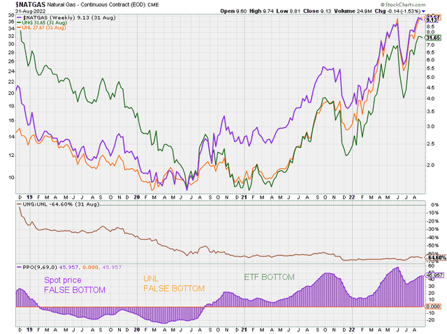
It is a typical however not inevitable setup. Spot costs momentum usually experiences a dramatic double dip in a downcycle. As soon as spot costs do backside, usually on that second strive, they usually explode upwards, however due to the steep contango, the ETFs won’t usually be well-positioned for it, particularly UNG, until you realize exactly the place to enter and exit.

In a typical cyclical transition, one of the best you possibly can hope to do is to catch the center of the upcycle (on this case, the 21Q1 backside to, realistically, the 21Q4 pullback while you panicked and bought). Throughout these phases of the upswing (for instance, 21Q1-21Q4 or 21Q4-22Q2), UNG outperforms UNL, nevertheless it quickly loses floor through the inevitable pullbacks.

What makes this doable is the mixture of rising momentum within the spot worth and a flattening of the futures curve, as illustrated within the chart beneath.

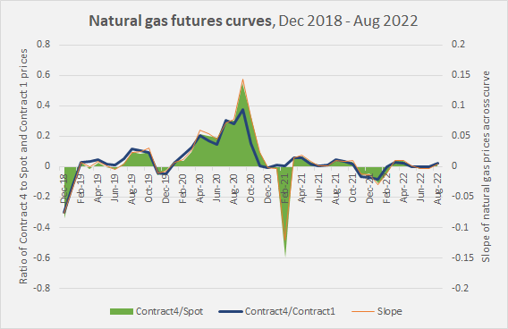
I’ve not calculated a exact cutoff level for the place the “proper” curve ought to be, however it seems that the ratio between Contract 4 and spot costs ought to be beneath the ten% degree (beneath 0.1 on the left-hand scale) and beneath 5% is significantly better.

The 2012-2014 upcycle

Should you take a look at the 2012-2014 cycle, you possibly can see comparable dynamics at work.

Discover that the UNG/UNL ratio within the center panel seems to be correlated with momentum within the spot worth illustrated within the backside panel. That’s largely as a result of the contango was comparatively gentle over a lot of this era.

One of many perversities of those relationships is that one of the best time to purchase into these ETFs is close to the conclusion of the upcycle, as momentum spikes and the longer term curves invert.

So, the place are situations now?

Present situations

First, we are able to take a look at the futures curve. The next chart exhibits spot costs (in black) and October 2023 (AKA Contract 4, in inexperienced) to February 24 contracts.

And the next chart exhibits the ratios of these contract to identify costs.

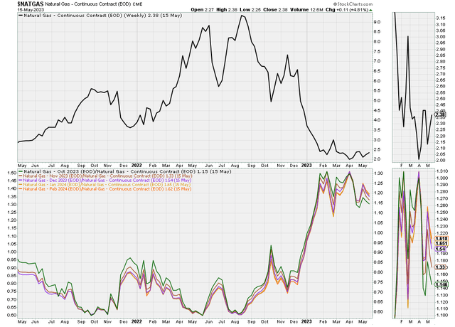
The October 2023 contract is 15% greater than spot costs, which is traditionally a bit too excessive to be enticing.

Momentum seems to be bottoming, nevertheless.

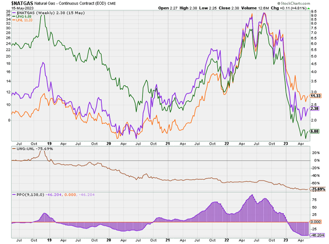
In sum, on the plus facet, the character of the commodity cycle, significantly the mixture of excessive gold costs and low pure gasoline costs, factors to the chance that we are going to see greater pure gasoline costs in 2024, maybe considerably greater. And, the obvious bottoming in momentum at present means that flip could be quickly upon us.

Conclusion

Pure gasoline’s volatility makes it doable for ETFs like UNG to double in a month’s time, however this appears to be very tough to time, and due to the character of those merchandise and the futures market they’re primarily based on, timing is every little thing.

Pure gasoline costs are more likely to be greater by the top of 2024 than they’re now, and it’s doable that for these eager on getting cash within the pure gasoline house, there will probably be alternatives to make use of these ETFs to take action, however it should in all probability be greatest to attend for extra propitious alternatives to take action, significantly when the ratio between Contract 4 and spot costs is beneath the ten% degree, and momentum in spot costs is on the rise.

For many who are however eager to achieve publicity to a possible pure gasoline upswing within the close to time period, in gentle of the state of the futures curve, it will in all probability be higher to purchase UNL for from time to time look forward to the futures curve to flatten. As soon as it has flattened and momentum turns up once more, UNG may present higher upside potential. And, then it should require every day vigilance, as as soon as that upward momentum breaks, the autumn could be terribly precipitous.

Timing these elements accurately might probably yield vital returns, however buyers ought to all the time concentrate on the dangers concerned and take into account their very own funding targets and danger tolerance earlier than investing in these risky ETFs.